
Table of Contents
What will we Learn from This Blog?
From this blog We will Learn About Excel AND Function and will be able to answer the Question “how to use AND function in excel” and Also “how to use the and function in excel”. The syntex of this function , How to Use it, All the Common Mistake of it, the Advance Tips and Tricks of it. Hope so we will end the blog and Know this Logical Function Thoroughly
Introduction
Importance of Functions in Excel
Excel is becoming a Day to Day Go through software now in this world, it uses to calculate, getting track of previous data. The functions are playing a crucial role in Excel as they enhance the efficiency and accuracy of data analysis and manipulation of data. From Automating Calculations, Dynamic Updates, Error Checking To data analysis it makes our life easy in everyday life.
Importance of Excel AND Function:
- Logical Testing: In excel AND function is used for checking multiple conditions simultaneously.
- Efficiency: The Function Simplifies the complex formulas and also nested IF statements.
- Error Reduction: It used to Minimize the risk of false positives or incorrect outcomes.
- Data Validation: Ensures data meeting specific criteria for accuracy.
- Consistency: Tt Handles multiple conditions and helo in maintaining data consistency.
What is the AND Function in Excel?
Defination
In Excel AND function is a logical function that returns TRUE only if all specified conditions within the function are met. It evaluates multiple arguments, and the result is TRUE only when all conditions are true.
Purpose
Purpose of using AND function in Excel is to perform the logical testing and also decision-making. It is used to check if multiple conditions are simultaneously satisfied. It Also allows users to create more complex and precise criteria for data analysis, validation, and efficient formula construction
Syntex of Excel AND Function:
Syntex
for AND Function Excel have syntex like:
=AND(logical1, [logical2], …)
- logical1: The first condition or expression to evaluate.
- [logical2], …: Additional conditions or expressions (up to 255 total) that you want to test. You can include multiple logical arguments separated by commas
The conditions can check things like:
- If a number is greater than another number >
- If a number is smaller than another number <
- If a number or text is equal to something =
Return Value
In Excel AND Function returns TRUE if all specified conditions are true; otherwise, it returns FALSE.
How to Use:
In Excel AND Function uses for evaluating multiple logical conditions, allowing for testing up to 255 conditions presented as arguments. Where Each argument, denoted as logical1, logical2, etc., should represent an expression producing either TRUE or FALSE or a value that can be interpreted as such. The arguments have a range of possibilities, including constants, cell references, arrays, or logical expressions.
Examples with Description
lets learn AND with Example:
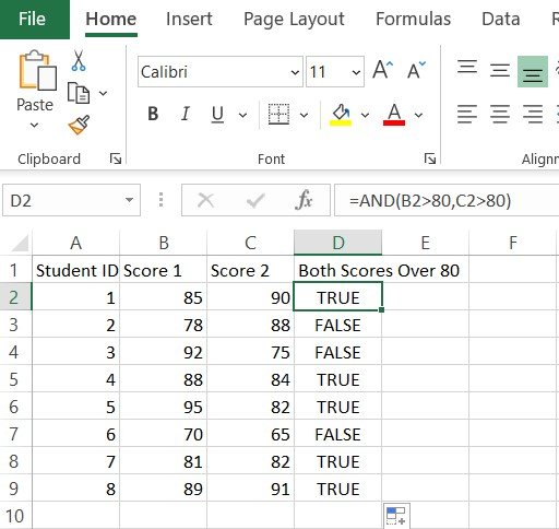
Problem 1: We have two Column, we have to return TRUE when Both the column have score over 80.
=AND(A2>80, B2>80)
Explanation:
A2>80: This argument Checks if the First Column have (in cell A2) is above 80
B2>80: Ensures that the First Columns value (in cell B2) is also above 80.
The AND function combines these conditions. If both conditions are true, the formula returns TRUE, Otherwise it will Show FALSE.
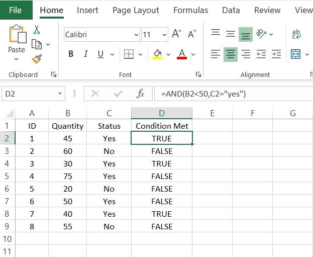
Problem 2: When One column Have Number in it and Other column have A text in it. We have to Return TRUE when the first Column have less value then certain limit and the second column have a fixed text.
=AND(A2<50, B2=”Yes”)
Explanation:
A2<50: Checks if the Number (in cell A2) is below 50 units.
B2=”Yes”: Ensures that the value (in cell B2) is set to “Yes.”
The AND function evaluates these conditions. If both are true, the formula returns TRUE
Problem 3: In a Certain scenario, certain Block (Column A) can only start if both the other block (Column B) is completed and the third block (Column C) is confirmed.
=AND(B2=”Completed”, C2=”Available”)
Explanation:
B2=”Completed”: Checks if the Block (in cell B2) is marked as “Completed.”
C2=”Available”: Ensures that the required the Block to be (in cell C2) is confirmed.
The AND function assesses these conditions. If both are true, the formula returns TRUE

Common Mistakes
Common Error:
Here are common errors associated with the AND function in Excel applications like Excel or Google Sheets, along with explanations:
Incorrect Syntax:
- Error: Using incorrect syntax such as missing parentheses or commas.
- Explanation: The AND function requires the format
=AND (conditions1,condition2,….). Ensure all conditions are separated by commas and enclosed within parentheses.
Non-Boolean Arguments:
- Error: Passing non-boolean values (text, numbers) without a logical condition.
- Explanation:in Excel AND function expects logical tests that evaluate to TRUE or FALSE. Using values like “text” or plain numbers without a comparison will cause errors. For example, =AND(“text”, A1 > 5) is incorrect.
Reference Errors:
- Error: Referencing cells that contain errors (e.g., #N/A, #DIV/0!).
- Explanation: If any argument in the excel AND function references an error value, the entire function will return an error. Ensure all referenced cells are error-free.
Empty Arguments:
- Error: Including empty arguments in the function.
- Explanation: The AND function requires valid logical conditions. Empty arguments can cause unexpected results or errors. Verify that all conditions are properly defined.
Overlooking Cell References:
- Error: Incorrectly referencing cell ranges or individual cells.
- Explanation: Ensure cell references are correct and within the intended range. Misreferences can lead to incorrect evaluations.
Mismatched Data Types:
- Error: Comparing mismatched data types (e.g., text with numbers).
- Explanation: Logical conditions should compare compatible data types. For example, comparing a text value to a number will not work as intended.
Function Nesting Issues:
- Error: Improperly nesting other functions within AND.
- Explanation: When nesting functions within AND, ensure each nested function returns a boolean value. Misnests can lead to formula errors.
How to solve
Here are solutions to the common errors associated with the AND function in spreadsheet applications:
Incorrect Syntax:
- Solution: Ensure the correct format =AND(condition1, condition2, …). Verify all conditions are separated by commas and enclosed in parentheses. For example: =AND(A1 > 5, B1 < 10).
Non-Boolean Arguments:
- Solution: Use logical conditions that evaluate to TRUE or FALSE. Convert plain text or numbers into logical comparisons. For example, instead of =AND(“text”, A1 > 5), use =AND(A1 = “text”, A1 > 5) if A1 is supposed to contain the text.
Reference Errors:
- Solution: Check and correct any errors in the referenced cells. Make sure none of the cells referenced by the AND function contain errors like #N/A or #DIV/0!. Use functions like IFERROR to handle potential errors in cell references.
Empty Arguments:
- Solution: Ensure all arguments are filled with valid logical conditions. Avoid leaving arguments empty. For example, instead of =AND(A1 > 5, , B1 < 10), ensure every condition is complete: =AND(A1 > 5, A2 < 15, B1 < 10).
Overlooking Cell References:
- Solution: Double-check all cell references to ensure they are correct and within the intended range. Correct any misreferences and make sure they point to the correct cells. For instance, =AND(A1 > 5, B1 < 10) should reference A1 and B1 as intended.
Mismatched Data Types:
- Solution: Make sure you compare compatible data types. For example, if comparing text, use text conditions: =AND(A1 = “Yes”, B1 > 10). Ensure text comparisons are enclosed in quotes and number comparisons are numerical.
Function Nesting Issues:
- Solution: When nesting functions within AND, make sure each nested function returns a boolean value (TRUE or FALSE). Correctly nest functions like =AND(ISNUMBER(A1), B1 < 10), ensuring each nested function (like ISNUMBER) correctly outputs a boolean.
By implementing these solutions, you can resolve the errors and ensure the AND function operates correctly in your spreadsheets.
How to Avoid
To avoid common errors when using the AND function in excel applications, follow these best practices:
Correct Syntax:
- Tip: Always check your syntax for proper formatting. Use the formula bar to ensure you have =AND(condition1, condition2, …). Ensure all conditions are separated by commas and the entire set of conditions is enclosed in parentheses.
Use Boolean Arguments:
- Tip: Make sure all arguments are logical tests that evaluate to TRUE or FALSE. Convert plain text or numbers into logical comparisons. For example, =AND(A1 > 5, B1 < 10) instead of =AND(“text”, A1 > 5).
Avoid Reference Errors:
- Tip: Before using cell references in your AND function, ensure those cells do not contain errors. You can use the IFERROR function to manage potential errors, such as = AND (IFERROR (A1 > 5, FALSE), IFERROR(B1 < 10, FALSE)).
Fill All Arguments:
- Tip: Ensure all logical conditions in the AND function are specified and not left empty. Verify that every condition is meaningful and complete. For example, use =AND(A1 > 5, B1 < 10) instead of leaving any argument blank.
Verify Cell References:
- Tip: Double-check all cell references for accuracy. Make sure you are referencing the correct cells and ranges. This can be done by clicking directly on the cells when constructing your formula to ensure proper referencing.
Match Data Types:
- Tip: Ensure comparisons are made between compatible data types. For instance, compare numbers to numbers and text to text. For example, use =AND(A1 = “Yes”, B1 > 10) for text and numerical comparisons.
Properly Nest Functions:
- Tip: When nesting functions within the AND function, ensure each nested function returns a boolean value (TRUE or FALSE). Verify each nested function individually before combining them. For instance, use =AND(ISNUMBER(A1), B1 < 10) where ISNUMBER(A1) must return TRUE or FALSE.
By following these tips, you can avoid common errors and ensure that your AND function operates correctly and efficiently in your spreadsheets.
Advance tips and Tricks:
Though it seams easy to work with Such Logical Functions, there are some Advanced Tips and Tricks that can elevate your spreedsheet journey even better. here are some tips given bellow:
Nesting AND Functions:
Tip: Combine Multiple AND Functions for Complex Conditions
=AND(AND(B2>100, C2>=20, C2<=30), D2=”Passed”)
By nesting multiple AND functions, you can handle more complex logic. This formula checks if:
- Cell B2 is greater than 100.
- Cell C2 is between 20 and 30 (inclusive).
- Cell D2 equals “Passed”.
If all conditions are met, the formula returns TRUE; otherwise, it returns FALSE.
Dynamic Cell References
Tip: Utilize Dynamic References for Changing Data Sets
The INDIRECT function allows you to create dynamic references, making it possible to change the target cells without modifying the formula. This is particularly useful in scenarios where data locations are subject to change.
Array Formulas with AND
Tip: Leverage Array Formulas for Multiple Cell Ranges
=AND((A1:A10>50)*(B1:B10=”Approved”))
Array formulas evaluate multiple cell ranges simultaneously. This formula checks each row within the ranges A1 and B1. If all conditions are met across the range, it returns TRUE. For use, enter the formula and press Ctrl+Shift+Enter.
Conditional Formatting with AND
Tip: Apply AND Function in Conditional Formatting
=AND(A1>10, B1=”Complete”)
Using AND in conditional formatting lets you visually highlight cells meeting specific criteria. For instance, this rule can color cells where A1 is greater than 10 and B1 is “Complete”, aiding quick data analysis.
Use of Named Ranges
Tip: Enhance Readability with Named Ranges
=AND(MonthlyRevenue>100000, YearlyProfitMargin>0.2)
Named ranges improve formula readability and manageability. Instead of using cell references, you use descriptive names. This makes your formulas easier to understand and maintain.
Incorporating IF Statements
Tip: Combine AND with IF for Customized Outcomes
=IF(AND(A1>10, B1=”Complete”), “Achieved”, “Incomplete”)
Combining AND with IF lets you customize outcomes based on conditions. If A1 is greater than 10 and B1 is “Complete”, it returns “Achieved”; otherwise, it returns “Incomplete”. This adds flexibility to your data handling.
Frequently Asked Questions
01. What does the AND Function Excel do Work?
The AND function in Excel returns TRUE if all specified conditions are true, and FALSE otherwise
02. How to use AND Function in excel?
The syntax is: = AND (logical1, [logical2], …)
03. How many conditions can I include in the Excel AND function?
You can include up to 255 conditions in the Excel AND function.
04. Can the Excel function AND be nested?
Yes, you can nest AND functions to evaluate multiple sets of conditions.
05. Does the AND functions support text or numerical values?
The AND function primarily works with logical values (TRUE/FALSE), but it can also handle text and numerical values.
06. What happens if I include empty cells or cells with errors in the AND functions?
If any argument is an empty cell or contains an error, the AND function returns FALSE.
07. How does the AND functions differ from the OR functions?
The AND function returns TRUE only if all conditions are true, while the OR function returns TRUE if at least one condition is true.
08. Can I use cell references as arguments in the AND functions?
Yes, you can use cell references as arguments to dynamically evaluate conditions based on the content of other cells.
09. Is the AND function case-sensitive?
No, the AND function is not case-sensitive, so it treats uppercase and lowercase text as equivalent.
10. Any tips for troubleshooting issues with the AND functions?
Check each logical condition separately, and ensure that there are no empty cells or errors in the arguments. Use parentheses for clarity when nesting multiple conditions.
For anymore queries you can Contact Through the given mail in Contact us